Contents

- Contents
- Previous
- Next
- Up
- Top of page
- 1. Download the signals
- 2. Unpack the archive
- 3. Launch geopsy
- 4. Load the demo signals
- 5. Create a table of signals
- 6. Modify the list of visible fields
- 7. Extract the component
- 8. Construct the station names
- 9. Set station coordinates
- 10. Creating the database on disk
- 11. Creating groups
- 12. Saving changes
3.1 Creating a database
This tutorial helps you constructing the demo database used in tutorials 3.3 and 3.4. It is divided into the following steps:
- 1. Download the signals
- 2. Unpack the archive
- 3. Launch geopsy
- 4. Load the demo signals
- 5. Create a table of signals
- 6. Modify the list of visible fields
- 7. Extract the component
- 8. Construct the station names
- 9. Set station coordinates
- 10. Creating the database on disk
- 11. Creating groups
- 12. Saving changes
This tutorial has been updated for geopsy 2.0.0-cvs-20051116. A stable release will be available once Qt 4.1 will be released.
1. Download the signals
Download the raw signals: database-step0.tar.gz. These signals were generated with HISADA code (Hisada 1994 and 1995) within the framework of the SESAME European Research project (Bonnefoy-Claudet 2004, SESAME). The reference model used to generate these signals is detailed in Wathelet 2005 (Model description).
2. Unpack the archive
Open a terminal and execute the following commands (note: "mwathele@Canucks:~$" is my bash prompt). Keep this terminal open until the end of this tutorial. Under Windows, double-click on the downloaded archive, and copy directory "geopsy_tutorials" to another location (e.g. "My documents").
| Unpacking the raw signals and the list of station coordinates |
mwathele@Canucks:~$ tar xvfz database-step0.tar.gz ... |
3. Launch geopsy
Geopsy can be started from the terminal or from the platform specific menu used to start new applications: KDE or Gnome menus, 'Startup' for Windows,... The exact name and the availability of the shortcut depends upon your installation parameters. Double-clicking on geopsy icon is also a possible method (geopsy.exe for Windows explorer or geopsy for Konqueror).
| Starting Geopsy's main frame |
mwathele@Canucks:~$ geopsy& |
Check your configuration, specified in the installation manual, if geopsy fails to start. If it is the first time you execute geopsy, you should see a splash screen and a first dialog box entitled "Preferences". At this stage, click on "OK" to accept the default settings.
4. Load the demo signals
Click on menu "File" and select "Import signals" item, or alternatively hit CTRL+L, or click on "Import signals" icon from the tool bar ( ). Change the current directory to "geopsy_tutorials/raw_signals". Select all files from "demo_01A.1.sac" to "demo_10A.3.sac" (with mouse and SHIFT key). Click on "Open" to proceed with the loading of files. If you get a dialog box asking for the format, make sure to select "Automatic recognition" and to unckeck "Show this dialog next time" before clicking on "OK". After a short delay (waiting for the progress bar at the bottom right to increase up to 100%), the loaded signal should appear on the left in the Files/Groups list. If not, please refer to the specialised sections or use the search engine of this documentation.
Note: at this stage, the signals are loaded into memory. For the purpose of this tutorial, the components, the station names, and the coordinates of the stations have been cleared from the SAC headers. Adjusting these fields is a common task for signals acquired on stations that do not record the required information. During the next step, you will learn how to set these fields in a rational way.
5. Create a table of signals
Click on "All signals" in the "Files" list. Drag and drop this item to the "Table" icon from the tool bar ( ). To drag and drop signals, press the left mouse button on the selected signals move the pointer to the desired destination, and release the left mouse button. Possible destinations are:
The three first destinations will create new viewers with the selected signals. The last destination will add the selected signals to the existing viewer. If the signals are dropped on a table, a table should appear with header information of all loaded signals, as shown in figure 1.
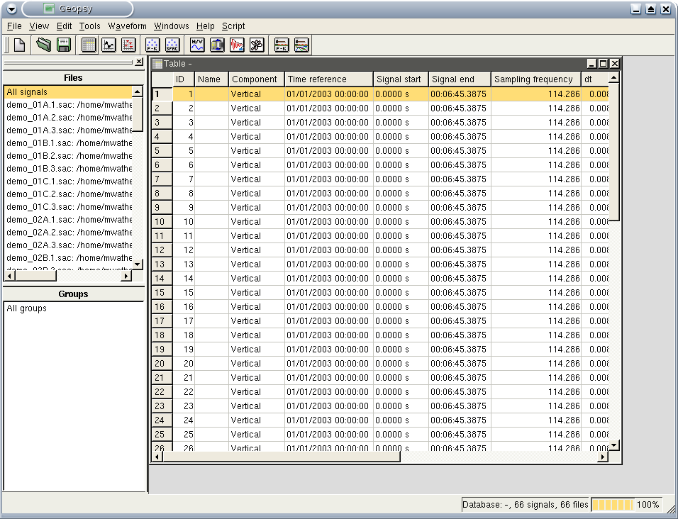
Figure 1: Table containing all loaded signals, empty headers.
The headers contain only the basic signal information: sampling frequency and number of samples. Other fields (such as the component) have been set to default values for all signals.
6. Modify the list of visible fields
Click on menu "View" and select "Set data fields" item. A dialog box as shown in figure 2 lets you modify the information displayed in the current table.
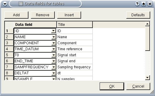
Figure 2: Dialog box that lets you modify the information displayed in tables.
In the left column, you have the names of the internal variables. On the right, you have the associated title in the table. Replace one of the useless fields (for this tutorial, e.g. "ID"), by the name of the file ("FileName"). Make sure (for the next steps) that the fields "SignalName", "Component", "ReceiverX", "ReceiverY", and "ReceiverZ" are in the list. Click on "OK" to apply the changes to the current table. The complete names of each signal should appear in the table.
7. Extract the component
The component is extracted from the signal file names. The components were stored in the file name structure with a number from 1 to 3, meaning Vertical, North, and East, respectively. Click on menu "Edit" and select "Set headers" item. A dialog box as shown in figure 3 lets you modify the header information by the means of a series of user defined equations.
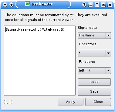
Figure 3: Dialog box that lets you modify header information
of each signal contained in the current viewer.
The white area containing the formulas is empty when you open this dialog box for the first time. Type your equation int the text area, eventually with the help of the lists on the right (Internal varaiables, Operators and Functions). More than one equation at a time can be entered, sepearating them by ";". Brackets may be used to group operations.
| Equation to extract the component indexes from the file names |
SignalName=right(FileName,5); |
Alternatively, you can download the file getcomp.headequ to load the equation. Click on "Load" and select the downloaded file. Click on "Apply" to execute the equation on the signals of the current table.
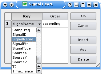
Figure 4: Dialog box that lets you sort the signal in a viewer.
Sort the signals by "name" to group the same components together. Click on menu "Edit" and select "Sort" item. A dialog box as shown in figure 4 lets you re-order signals in the current viewer according a series of user-defined keys. Click on "Add" to add a new sort key. If the list of keys was not empty, first remove all items by clicking on "Delete". The position within the list is important, the first item is the main sort key. Change the key type by clicking in the first column and select the right key. You can change the order in the second column. Click on "OK" to re-order the signals in the current table (or attached viewer).
Select all the signals with the name equal to "2.sac". Drag and drop these signals to the table icon (). Click on menu "Edit" and select "Set headers" item to modify the "Component" field for the signals of the newly created table. Enter the following equation or load the file setnorth.headequ:
| Equation to set component as North |
Component="North"; |
Once the components are changed, close the current table and go back to the first table containing all the signals. The same job must be done for "3.sac" (corresponding to East components). Enter the following equation or load the file seteast.headequ:
| Equation to set component as East |
Component="East"; |
The content of the main table is refreshed automatically after any changes performed in another table.
8. Construct the station names
Click on menu "Edit" and select "Set headers" item to modify the "SignalName" field of all signals. Enter the following equation or load the file setnames.headequ:
| Equation to set the station names |
SignalName = "R" + left ( right( FileName, 9 ), 3 ) ; |
9. Set station coordinates
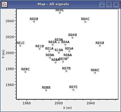
Figure 5: Station map
Click on menu "Edit" and select "Set receivers" item to set the receiver coordinates. A dialog box will display the list of station names with the coordinates X, Y, and Z. Click on "Load" to load the coordinate file receivers.coord. This operation adds new rows in the station list. The added station names should be identical to the existing names to overwrite the current coordinates. By clicking on "OK", the coordinates of the signals are modified. To check them, a map of the station can be viewed be dragging "All signals" to the map icon ( ). The result should look like in figure 5.
10. Creating the database on disk
Click on menu "File" and select "Create database" item. You will be prompted for a database name. A directory will be created and information will be saved inside this new directory. Creating a database allows you to create groups of signals as described in the next step.
11. Creating groups
Make sure that the map created in step 9 is currently active. Right click in middle of the map to display the context menu and select "Edit" item or alternatively hit CTRL+SHIFT+e. If no "Edit" item is present in the context menu it is likely that you right click at the wrong place. Four distinct areas are present on such XY graph: X axis, Y axis, bottom left corner and the graph's content. A "editing ..." message should appear on the plot. By pressing mouse left button and moving the pointer, you create virtual rectangles. All stations coordinates falling inside this rectangle are selected. To unselect all, construct a rectangle with no station inside. To add new selected station press SHIFT while pressing the mouse.
Three station array can be constructed from the ensemble of stations:
- One small circle with stations: R01A to R10A;
- Three triangle rotated by 120�: R10A, R03A, R06A, R09A, R01B to R08B;
- One big circle: R10A, and all stations on the big circle.
Select the stations of one array. The stations must appear in red. Hit CTRL+SHIFT+e to end the editing mode. Drag and drop the content of the graph to the table icon to create a new table. Click on menu "Edit" and select "New group" item. Enter a name for the group of signals (e.g. "array_A"). Close the table, and activate the map again. Go back to editing mode by hitting CTRL+SHIFT+e again. Unselect all stations and select another array. Other arrays should be named "Array_B" and "Array_C".
For conventional array analysis, the vertical component is often used without the North and East components. Special groups of signals with only the Vertical components can be created for each array, for instance, "Array_A Vertical", "Array_B Vertical" and "Array_C Vertical".
Right click on group "Array_A" in the "Groups" list on the left. Select the "Table" item to create a table containing only this group. Select "Sort" from menu "Edit". "Insert" sort key "Component" to re-order signals by components. Select only the signals with a Vertical component and drag it to the graphic icon ( ). Click on menu "Edit" and select "New group" item. Enter a name for the group of signals (e.g. "array_A Vertical"). Close all windows and redo the same task for arrays B and C.
12. Saving changes
Click on menu "File" and select "Save database" item. The groups and any modification to the signals are saved on the disk. The complete database can be downloaded database-step12.tar.gz. On opening this database, the path to the original files are certainly not correct. You will be warned as explained in Opening an existing database.
